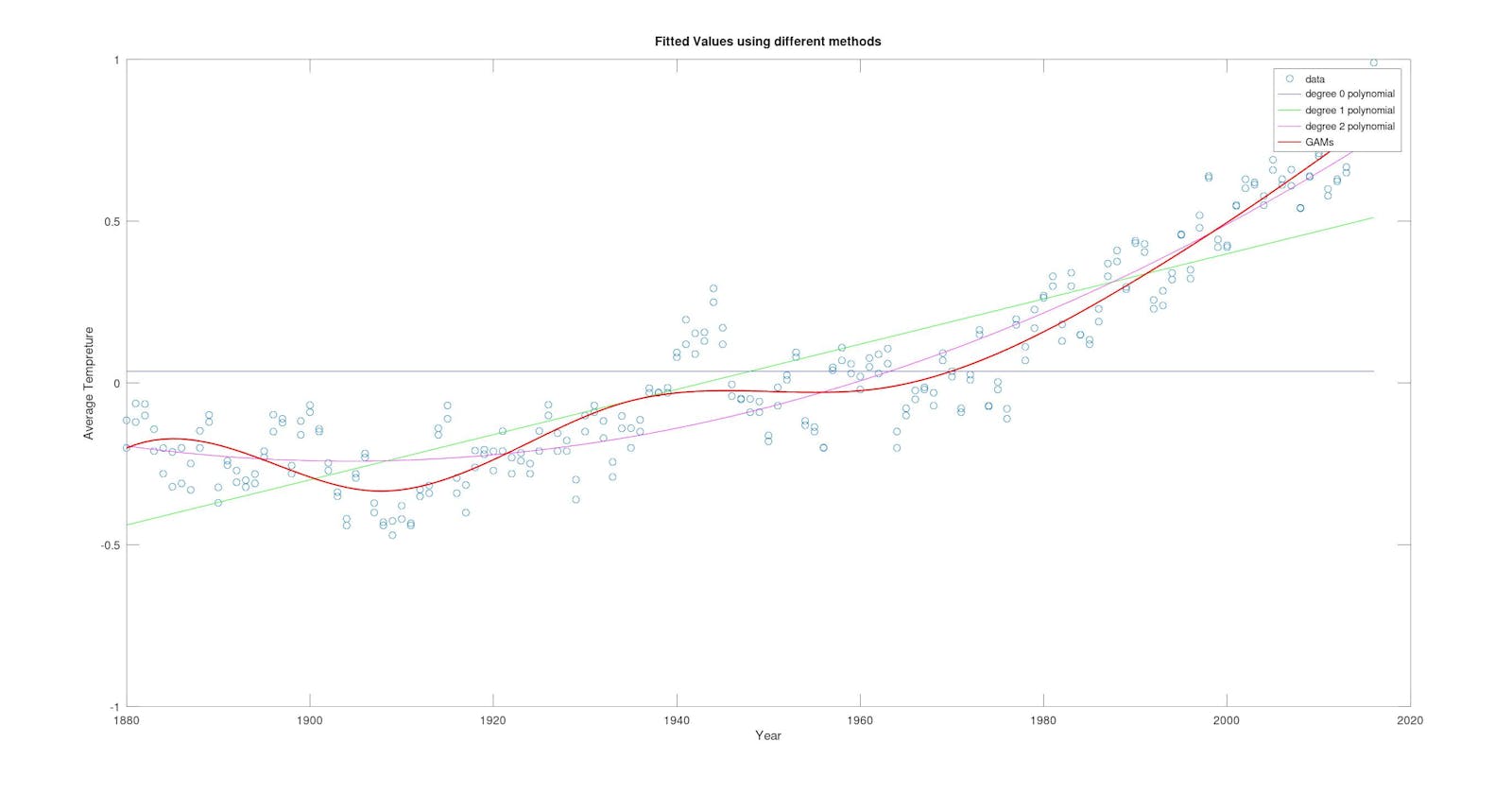
why GAMs ?

A Linear Model is Represented as :

$$Y=Xβ+ε$$

where Y is the Response Variable, X is the predictor data, Beta is the regression Coefficient, and epsilon is the error term. Linear models are known to be all-in-one models when it comes to data modeling. However, GLM are constricted by the assumption that the relationship between Response and predictor is linear, and the GLMs model this as such. although it's very simple, the real-life data are often not linear in relationship. With more complex data the GLMs might not be the best when it comes to modeling data. Let's have a look at the Average temperature every year from 1880 to 2016 from here.

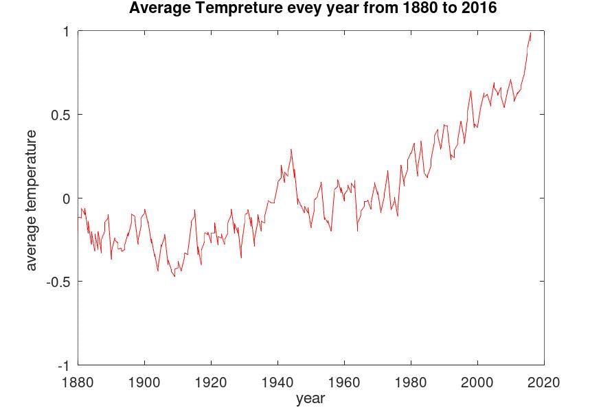
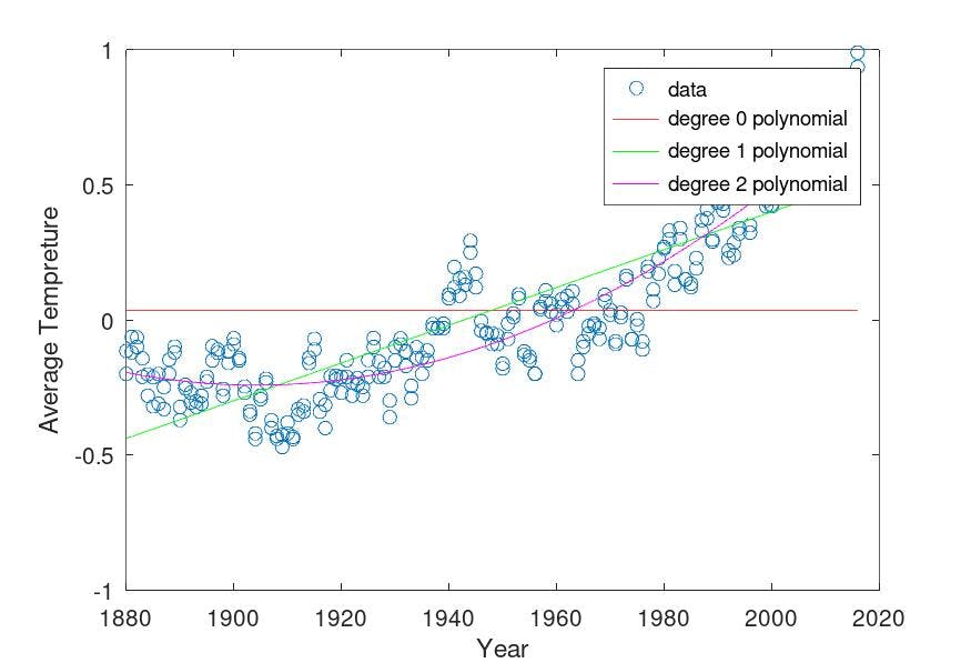
As we can see Fitting a simple line into this data will not result in better predictions, However, this can be overcome by fitting a polynomial of a higher degree.

Using Degree 1 and Degree 2 polynomial:

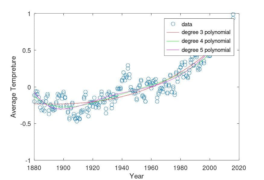
Degrees 3,4 and 5 :

using Higer order 10, 13, and 15 degrees:

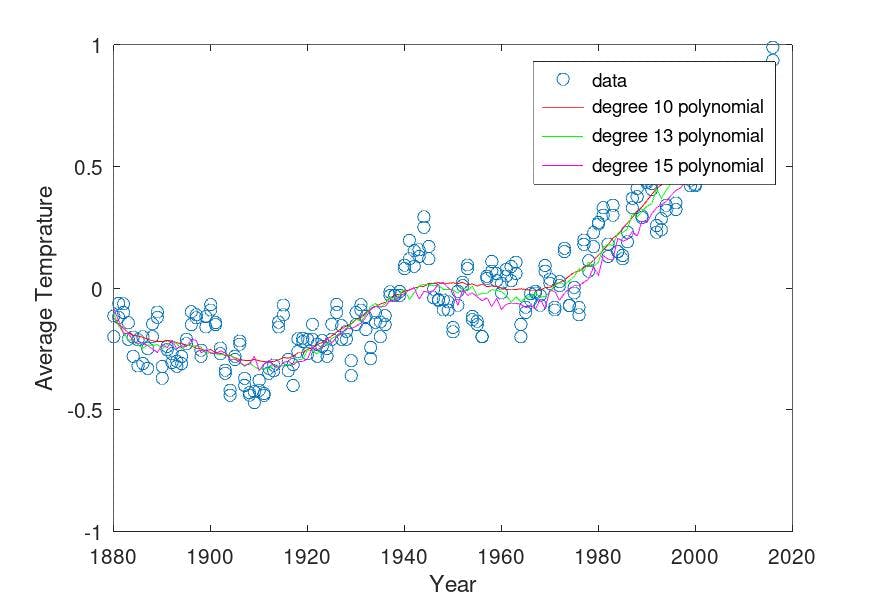
To model the outliers the Line is "wiggling" to capture the trends, This might look like it is doing a good job but actually the predictions are still bad and it doesn't account for all the dips and rises in the years particularly.

Now have a look at this :

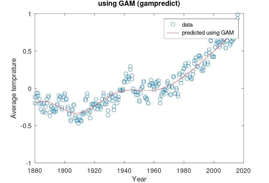
this is the predicted Temperature using GAMs ( gampredict function). The Predictions look actually good and capture the trends to appropriate degrees.

Generalized Additive Models (GAM)

GAMs can be defined as an adaptation that allows us to model non-linearity in the data maintaining the Linear models like interpretability.

A simple Multiple linear regression can be extended and represented as :

$$y_i = β_0+β_1x_{i_1}+β_2x_{i2} ​ +…+β_px_{ip} ​ +ϵ_i ​$$

In the regression setting, a generalized additive model has the form :

$$E(Y |X_1 , X_2 , . . . , Xp ) = α + f_1 (X_1 ) + f_2 (X_2 ) + · · · + f_p (X_p )$$

$$g(\mu) = b_0 + f(x_1) + f(x_2) + \ldots + f(x_p)$$

where g(μ) is the link function and f(x1),f(x2)....f(xp) are the Non-linear Function predictors for predictors X1, X2,.......Xp. The key difference here is instead of Smoothing term B0 to Bp, It now incorporates Smooth functions of the features (predictors), Represented as f(x), this will allow us to model Non-linear relationships between the predictor (x) and response (y).

Implementing GAM regression

GAMs were developed and introduced by R. Tibshirani and T. Hastie in 1984 as a blend of GLMs and additive models. The original paper can be found Here.

The Smoothing function f(x) can be shown to be a Spline which are piecewise polynomial function with continuous 2nd derivatives. Fitting each predictor with a spline will model the non-linear data.

In the Original paper, a Backfitting algorithm is suggested to fit a GAM.

Back fitting algorithm:

$$Initialize : \hat{\alpha} = \frac{1}{N} \sum_{i=1}^{N} y_i, \hat{f}_j \equiv 0, \forall i, j.$$

$$\text { Cycle: j = 1,2 .....p, 1,2.....p}$$

$$2 . \hat{f}j \leftarrow \frac{1}{N} \sum{i=1}^{N} \hat{f}j (x{ij}).$$

$$\text {Repeat 1 and 2 Until convergence is reached}$$

Implementation in Octave

Generating synthetic data, 100 samples for two functions with added noise:

## synthetic datasample
f1 = @(x) cos (3 *x);
f2 = @(x) x .^ 3;

samples = 100;

x1 = 2 * rand (samples, 1) - 1;
x2 = 2 * rand (samples, 1) - 1;

y = f1(x1) + f2(x2);
y = y + y .* 0.2 .* rand (samples,1);

X = [x1, x2];

For fitting a spline of degree 3, We would be using splinefit in Octave,

m = mean (y);
# calculate Residuals for first round of backfitting
res = y - mean (y);
RSS  =  0;
converged = false;
iterations  = 0;
ppf = struct();

while (! converged)
iterations += 1;

  for j = 1:columns (X)
    if ( itt > 1) #(i > 1)
     res = res + ppval (ppf (j), X (:, j));
    endif

    gk = splinefit (X (:,j) , res, 5, 'order', 3);

    gk.coefs = gk.coefs - sum (sum (gk.coefs)) / rows (X);

    RSSk (j) = abs (sum (abs (y - ppval (gk, X(:,j)) - m )) .^ 2) / rows (y)
    ppf (j) = gk;
    res = res - ppval (ppf (j), X (:,j));
  endfor
  if (all (abs (RSS - RSSk) <= tol))
    converged = true;
  endif
  RSS = RSSk;
endwhile