GSoC'23 Week 4: Implementing kNN algorithm for classification

GSoC'23 @ GNU Octave. Open-source software advocate
kNN Algorithm
in the parametric approach, we assume an underlying relationship between the predictor (input) and response (output) values.
$$Y = f(X, \theta) + \epsilon$$
Y represents the response variable, X represents the predictor variable(s), f represents the parametric model or function, \θ represents the parameters of the model that need to be estimated, and \epsilon represents the error term or random noise. This equation represents the relationship between the response variable and the predictor variable(s) in a parametric model, where the model function f is defined by the parameters \θ. The error term is \epsilon .
We simplify this equation by assuming f(x) takes a particular form (linear, polynomial etc..)
$$f(x_1,x_2...x_n)_{linear} = \beta_0 + \beta_1 X_1 + \beta_2 X_2 + \ldots + \beta_n X_n + \epsilon$$
$$f(x_1,x_2...x_n)_{polynomial} = \beta_0 + \beta_1 X + \beta_2 X^2 + \ldots + \beta_n X^n + \epsilon$$
the exact form of the model can be determined by the model's parameters
$$\beta_0,\beta_1,\beta_2...\beta_n$$
this is the Parametric Approach, this makes them more restrictive than nonparametric algorithms, but it also makes them faster and easier to train. Parametric algorithms are most appropriate for problems where the input data is well-defined and predictable. some examples of Parametric approaches are linear regression, logistic regression and Neural Networks.
this can be useful when we don't have a lot of data, as we reduce the problem of learning a completely unknown and arbitrary function f to learning the values of a handful of a parameters (p+1) betas.
In the Nonparametric approach, the algorithm is not based on a mathematical model instead, they learn from the data itself. This makes them more flexible than parametric algorithms but also more computationally expensive than parametric algorithms. Nonparametric algorithms are most appropriate for problems where the input data is not well-defined or is too complex to be modelled using a parametric algorithm.
Instead of assuming that function f takes a mathematical form, we assume that cases:
that have similar predictor values, must have similar response value
Let's try to understand the kNN algorithm with an example :
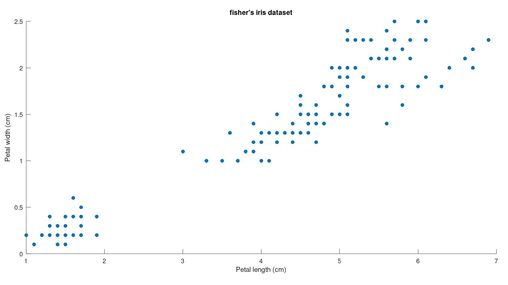
fisher's iris dataset contains data for the measurement of 150 different instances of flowers with each column corresponding to different measurements of flower parts and the species of the flower to which it belongs.
| Sepal length | Sepal width | Petal length | Petal width | Species |
| 5.1 | 3.5 | 1.4 | 0.2 | I. setosa |
| 4.9 | 3.0 | 1.4 | 0.2 | I. setosa |
| 4.7 | 3.2 | 1.3 | 0.2 | I. setosa |
| ... | ... | ... | ... | ... |
| 7.0 | 3.2 | 4.7 | 1.4 | I. versicolor |
| 6.4 | 3.2 | 4.5 | 1.5 | I. versicolor |
| ... | ... | ... | ... | ... |
| 7.7 | 3.8 | 6.7 | 2.2 | I. virginica |
| 7.7 | 2.6 | 6.9 | 2.3 | I. virginica |
Visualising this data set :
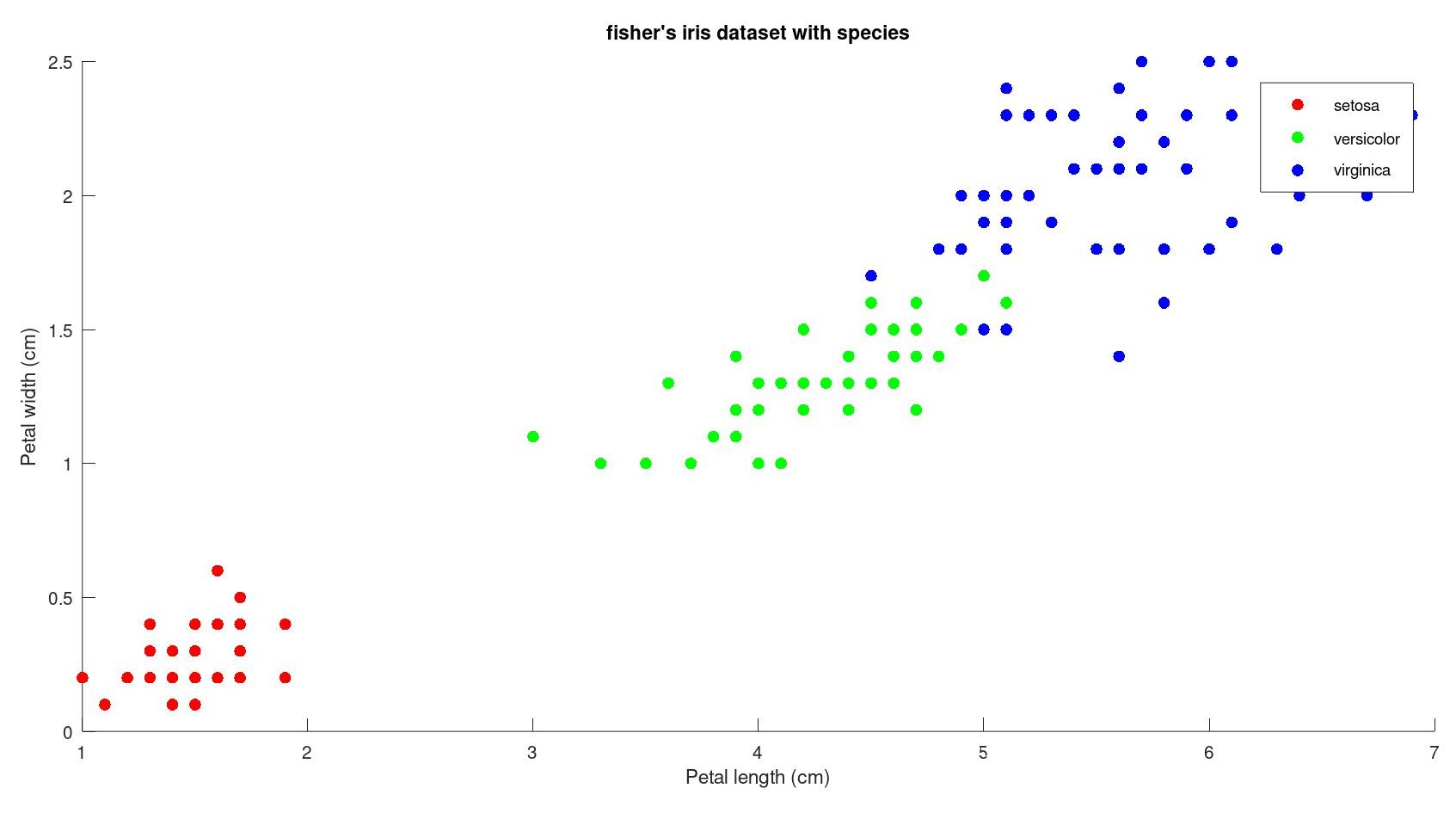
if we group them by species :
Let's only take petal data ie. petal length and petal width for all 150 observations of different flowers into account for simplicity. now let's say we record another observation of a new flower with petal length = 5 cm and petal width = 1.45 cm. How do we determine what species does it belong?
In kNN algorithm, we calculate the distance between the new observation and the existing data to determine the distance of the new observation from the existing observations. and count the number of nearest 'k' neighbours to which each of the k points belongs to. the species with the most nearest neighbour to the new observation will be the species of the new observation.
load fisheriris
x = meas(:,3:4);   ## consider only the petal length and width
y = species;       ## species matrix

point = [5, 1.45]; ## new observation
k = 10;
[id, d] = knnsearch (x, point, "K", 10);
gscatter(x(:,1), x(:,2), species,[.75 .75 0; 0 .75 .75; .75 0 .75], '.',20)
xlabel('Petal length (cm)');
ylabel('Petal width (cm)');
line (point(1), point(2), 'marker', 'x', 'color', 'k', 'linewidth', 2, 'displayname', 'query point')
line (x(id,1), x(id,2), 'color', [0.5 0.5 0.5],'marker', 'o', 'linestyle', 'none', 'markersize', 10, "displayname", "eulcidean")
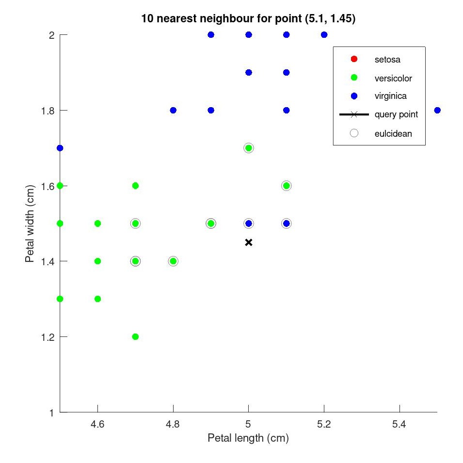
as we can see the point marked in 'x' has 10 nearest neighbours,
| no. of Nearest Neighbour | species |
| 6 | versicolor |
| 2 | Virginia |
6 belong to versicolor and 2 to Virginia species, by majority the new species belongs to the versicolor species of the flower.
Implementing knnpredict
knnpredict will take the predictor variable and species as mandatory variables and would take optional parameters as name-value pairs. where x will contain the data, y the classes of data that it belongs to and 'Xclass' new observations to be classified by the function.
additional arguments can be given as name-value pairs which include :
'K': number of nearest neighbours to be considered in kNN search.
'weights': numeric non-negative matrix of the observational weights, each row in WEIGHTS corresponds to the row in Y and indicates the relative importance or weight to be considered in calculating the Nearest-neighbour, negative values are removed before calculations if weights are specified.
'cost': numeric matrix containing misclassification cost for the corresponding I
'Cov': covariance matrix for computing Mahalanobis distance.
'bucket size' : maximum number of data points per leaf node of kd-tree.
'distance' is the distance metric to be used in calculating the distance between points. the choice for distance metric are : 'euclidean', sqeuclidean' , 'cityblock', 'chebyshev', 'minkowski', 'mahalanobis' , 'cosine', 'correlation' , 'spearman', 'jaccard' , 'hamming'.
'NSMethod': nearest neighbour search method. Choices for NSMETHOD are: - 'exhaustive' and 'kdtree'.
'standerdize': flag to indicate if kNN should be calculated by standardizing X.
the function knnpredict will return label, Score and cost
predicted labels can be calculated by minimizing the following function where nbd represents the neighbour points:
$$p(j\mid x_{\text{new}}) = \sum_{i \in \text{nbd}} \frac{W(i) \mathbf{1}{Y(X(i))=j}}{\sum{i \in \text{nbd}} W(i)}$$
The score is calculated:
$$\tilde{p_k} = \frac{p_k}{\sum_{k=1}^{k}p_k}$$
with observational weights
$$\tilde{w_j} = \frac{w_j}{\sum_{\forall j \in k }w_j}$$
posterior probabilities :
$$p(j\mid x_{\text{new}}) = \sum_{i \in \text{nbd}} \frac{W(i)1\{Y(X(i))=j\}}{\sum_{i \in \text{nbd}} W(i)}$$
and cost
$$\sum_{i=1}^{K} P(i\mid X_{\text{new}}(n)) C(j\mid i)$$
Code for knnpredict can be found here.
Implementing classdef for kNN
for Matlab compatibility and better representation of kNN model we will need a classdef ClassificationKNN for storing the training data and other model parameters.
A classdef should be in a separate folder with name @classdefname, this folder should contain the code for the classdef.
In Octave classdef has the following structure:
classdef classificationKNN
    properties (Access = private)
        property1;
        property2;
        .....
    endproperties

    methods (Access = public)
        function y = methods1 (params)
            ...
        endfunction
    endmethods
endclassdef
as the classdef implementation of octave is not complete, I have to mostly rely on existing classdef to implement new classdef.


